Linear Case Study

System model

Linear Case Study

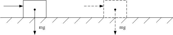
The system is a linear system. For a unit mass continuous time system, it is

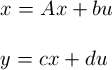
where x=[p v]', a=[0 1;0 0], b=[0 1]', c=[1 0], and d=0. For a unit mass discrete-time system, it is

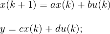
where x=[p v]', a=[1 T;0 1], b=[T^2/2 T]', c=[1 0], d=0. T is sample time, p is the position, and v is the velocity.

State-Feedback LQR (Linear Quadratic Regulation)

Synthesis:

The optimal state-feedback LQR is a simple matrix gain of the form 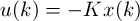, where K is the gain matrix and is given by Algebraic Riccati Equation (ARE). (In Matlab, we can use "[K,S,e] = dlqr(a,b,Q,R)" to get K). When Q=[0.1 0;0 0] and R=1, we get K=[0.3100 0.7874]'.

Result:

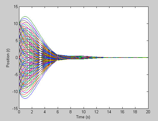Position

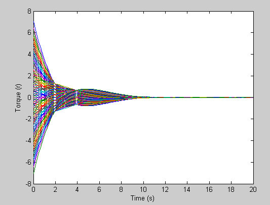Applied force for different initial state.

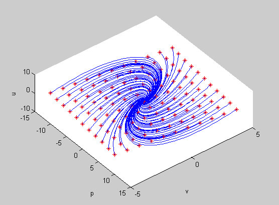Control policy. The trajectory (the blue lines) starts from the initial state (the red star) and terminates at the goal.

Trajectory Optimization

This problem can also solve by the optimizer. In AMPL, this problem can be written as

 
param init_xp :=10;
param init_dxp :=0;
param pi := 4*atan(1);
param N := 500;
param time := 20;
param dt := time/N;
param mass := 1.0;
param goal := 0;
param state_penalty := 0.1;
var x{0..N} >= -15, <= goal + 15;
var v_offset{i in 0..N-1} = (x[i+1]-x[i])/dt;
var v{i in 1..N-1} = (v_offset[i]+v_offset[i-1])/2;
var a{i in 1..N-1} = (v_offset[i]-v_offset[i-1])/dt;
var u {i in 1..N-1} >=-5, <=5, :=0.0;
minimize energy:
         sum {i in 1..N-1} (state_penalty*(x[i]-goal)*(x[i]-goal) + u[i]*u[i])*dt;
s.t. newton {i in 1..N-1}:
	u[i] = mass* a[i];
s.t. x_init: x[0] = init_xp;
s.t. x_final: x[N] = goal;
s.t. v_init: v_offset[0] = init_dxp;
s.t. v_final: v_offset[N-1] = 0;
let {i in 0..N} x[i] := init_xp+(goal-init_xp)*i/N;

Results:

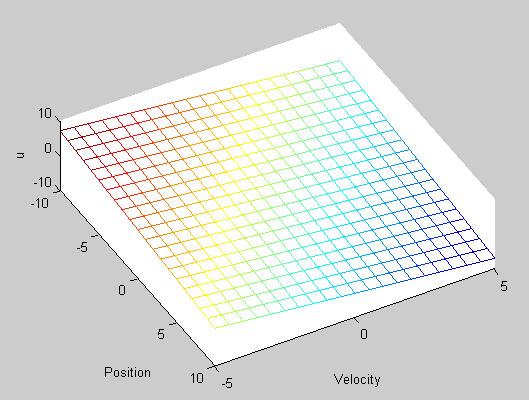Control policy