Dynamic Parameter Identification
Table of Contents
1 Introduction
Dynamic parameter identification is always compulsory for a real robot. However, a humanoid robot has many parameters and the process of determining these parameters a challenge problem1. Some link inertial parameters may not be identifiable due to the robot particular geometry. Reasons for unidentifiable parameters include restricted motion near the base and the lack of full force-torque sensing at each joint.
2 Methods
2.1 General Approach
In order to identify the dynamic parameters of an articulated robot, the robot model is formulated as:
where  is the joint torques,
  is
a
is
a  regressor matrix. The regressor matrix
  depends on the joint angles, velocities, and accelerations.
The Least-Square (SL) method is often applied in order to determine the inertial parameters. in general, it consists of the following several steps:
- Using the Newton-Euler formalism, generate a robot model that is linear in terms of the inertial parameters;
- reduce the inertial parameters set to a base set;
- determine the optimal trajectory parameters and optimize the excitation of the trajectories;
- estimate the link parameters using a standard least squares procedure.
2.2 Optimization Approach
In general, each link has 10 inertial parameters: its
mass, the position vector of its center of gravity with respect
to the base frame scaled by the link mass, 3 inertia moments,
and 3 inertia products. Thus, an n-link manipulator has 10n
dynamic parameters to be estimated. However,
for the planar robot model, each link has only
four parameters to be estimated:
its mass, the position vector of its CoM with respect to the base frame,
one inertia moment. Thus there are totally eight parameters for 2-link model.
There are some hoses and wires connected to Sarcos,
which apply external forces.
However, this external forces change slightly during experiments.
so we take them as a constant forces and additional parameters to be estimated.
which are  ,
,  ,
,  ,
,  .
.
The joint angles,  , can be measured directly, but the angle velocity,
  ,
and the angle acceleration,
,
and the angle acceleration,  , have to be numerically reconstructed.
The reconstructing filter does not work in real time and thus it can be anti-causal,
Therefore, a forward and reverse digital filtering can be used 2.
With the help of the inverse dynamic model, the joint torques and
the ground reaction forces can then be predicted.
Then we use these predicted values to fit the measurements, thus
the dynamic parameters can then be determined by the following
optimization problem:
, have to be numerically reconstructed.
The reconstructing filter does not work in real time and thus it can be anti-causal,
Therefore, a forward and reverse digital filtering can be used 2.
With the help of the inverse dynamic model, the joint torques and
the ground reaction forces can then be predicted.
Then we use these predicted values to fit the measurements, thus
the dynamic parameters can then be determined by the following
optimization problem:
where

and  are computed joint torque,
  are computed groud reaction force,
 is the corresponding measurement vector,
 is the push size measurement,
  is the push location,
 is a weighted matrix of diag(1,1,1,1).
3 Results
The following results are according exp0826
| m1 | m2 | x_m1 | y_m1 | x_m2 | y_m2 | MoI1 | MoI2 | x_f | z_f | f_x | f_z | |
| set1 | 56.39 | 37.36 | 0.14 | 0.56 | -0.07 | 0.62 | 1.24 | 1.73 | 0.01 | 0 | -8.49 | 3.81 |
| set2 | 55.99 | 36.76 | 0.15 | 0.77 | -0.05 | 0.61 | 1.23 | 1.16 | 0.02 | 0.58 | -7.43 | -8.4495 |
Fitting result
- set1 use 'e00118','e00120', save use_push_forward.mat
- set2 use 'e00124','e00126', save use_push_backward.mat
4 Discussion
4.1 Large fitting error
fitting data is e00120
Results:
para1 = [51.2111 41.9894 0.1533 0.8000 -0.0622 0.7294
1.2563 1.7681 -0.0648 0 -8.1618 5.9660]
data are saved in soft.mat
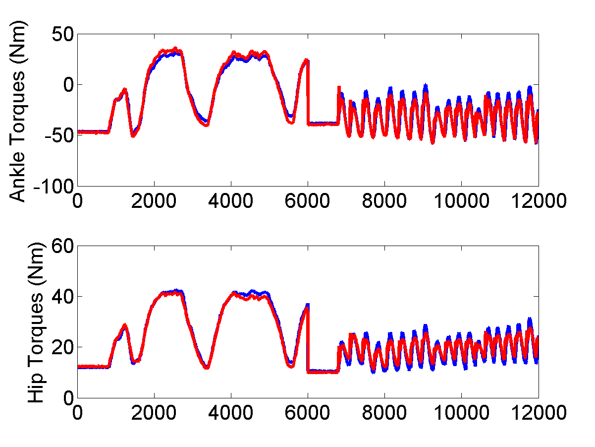
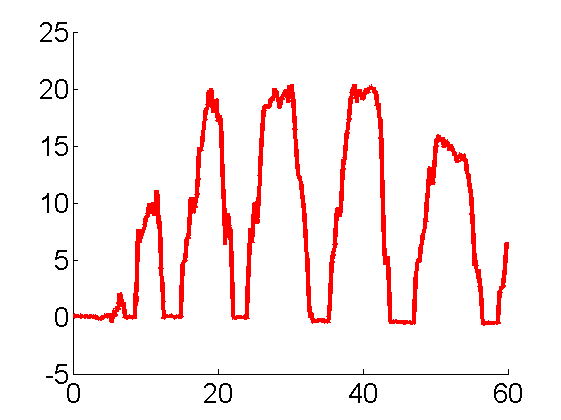
Measurements of push sensor
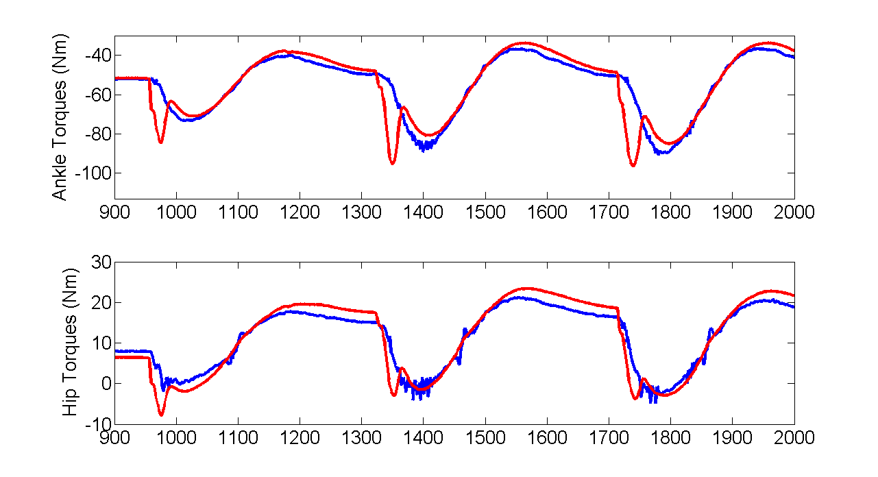
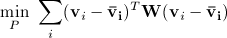
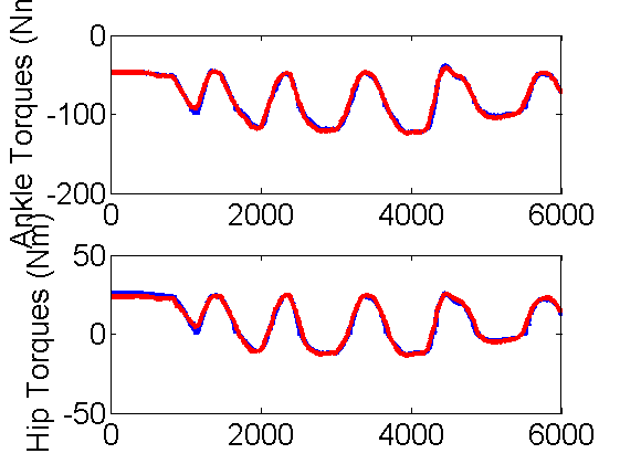
Measurements and fitting of joint torques
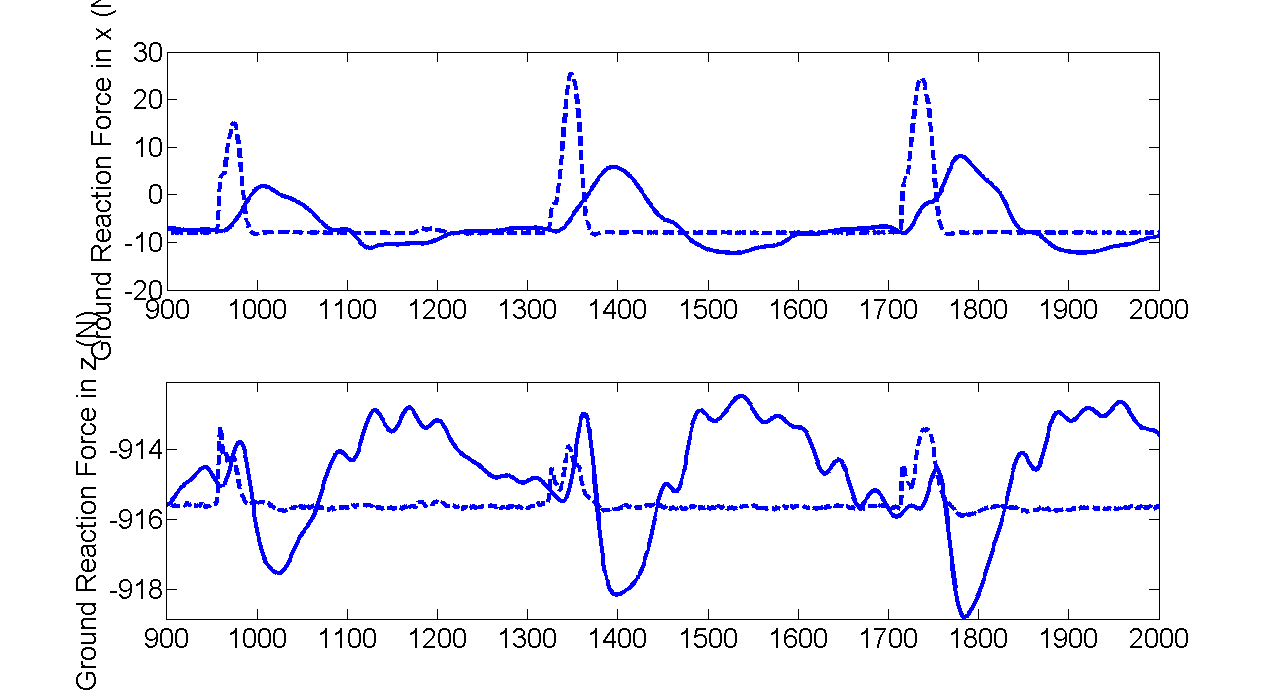
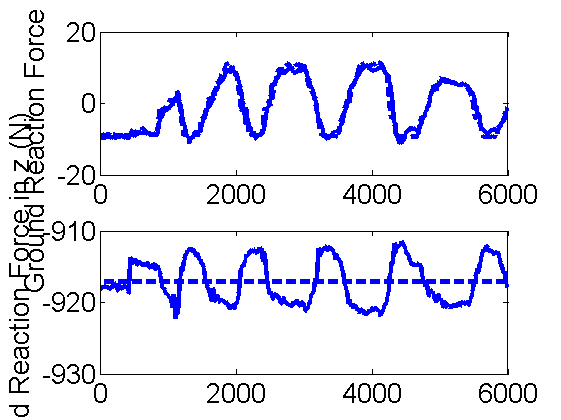
Measurements and fitting of the ground reaction force
There are large fitting errors when pushes are being applied. These errors may be caused by the arms and the knees movements, although they are almost fixed with high gain position controllers.
5 Consistent Results
In the following experiments, the identification results change with different data set.
5.1 Results
5.1.1 Slow forward pushes
- data file name: e00118
- para1 = [55.9898 37.7088 0.1448 0.3805 -0.0610 0.5543 1.2434 1.7304 0.0170 0.1477 -8.8264 2.0603]
- Fitting results
5.1.2 slow backward pushes
- data file name e00124 and result saved as use_e00124.mat
- para1=[56.0561 37.9955 0.1367 0.5658 -0.0630 0.6091 1.2434 1.7304 -0.0070 0.1237 -7.3292 4.1138]
5.1.3 fast forward pushes
- data file name e00120 and result saved as use_e00120.mat
- para1 = [53.1744 40.6310 0.1476 0.8000 -0.0641 0.7669 1.2437 1.7328 -0.0950 0.1923 -8.1619 4.7490]
5.1.4 fast backward pushes
- data file name e00126 and result saved as use_e00126.mat
- para1 = [51.9881 41.9272 0.1553 0.8000 -0.0560 0.7651 1.2437 1.7307 0.1521 0.3779 -7.5218 -0.0582]
5.1.5 Comparison
| Experiment Data | m1 | m2 | x_m1 | y_m1 | x_m2 | y_m2 | MoI1 | MoI2 | x_f | z_f | f_x | f_z |
|---|---|---|---|---|---|---|---|---|---|---|---|---|
| e00118(slow forward) | 55.9898 | 37.7088 | 0.1448 | 0.3805 | -0.0610 | 0.5543 | 1.2434 | 1.7304 | 0.0170 | 0.1477 | -8.8264 | 2.0603 |
| e00124(slow backward) | 56.0561 | 37.9955 | 0.1367 | 0.5658 | -0.0630 | 0.6091 | 1.2434 | 1.7304 | -0.0070 | 0.1237 | -7.3292 | 4.1138 |
| e00120(fast forward) | 53.1744 | 40.6310 | 0.1476 | 0.8000 | -0.0641 | 0.7669 | 1.2437 | 1.7328 | -0.0950 | 0.1923 | -8.1619 | 4.7490 |
| e00126(fast backward) | 51.9881 | 41.9272 | 0.1553 | 0.8000 | -0.0560 | 0.7651 | 1.2437 | 1.7307 | 0.1521 | 0.3779 | -7.5218 | -0.0582 |
| e00155(forward) | 41.4707 | 53.1944 | 0.1871 | 0.7351 | -0.0284 | 0.7703 | 1.2436 | 1.7310 | 0.0828 | 0.4283 | -10.0000 | 4.8583 |
| e00156(backward) | 40.7100 | 53.7653 | 0.1939 | 0.5666 | -0.0283 | 0.7871 | 1.2434 | 1.7404 | 0.1319 | 0.8000 | -10.0000 | 6.4235 |
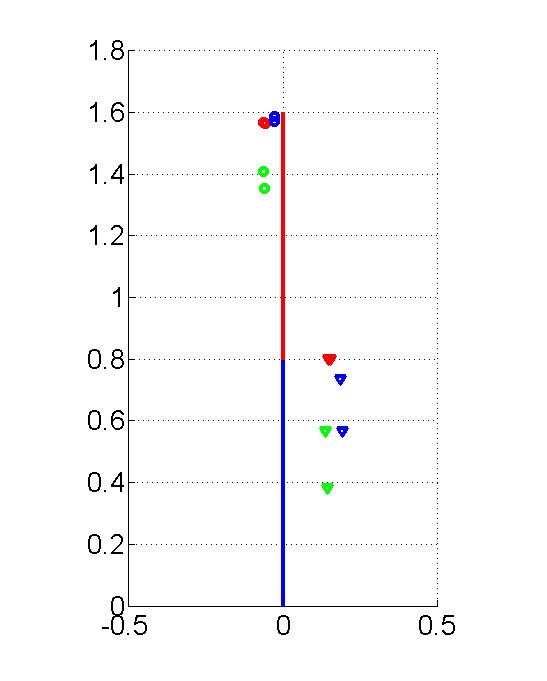
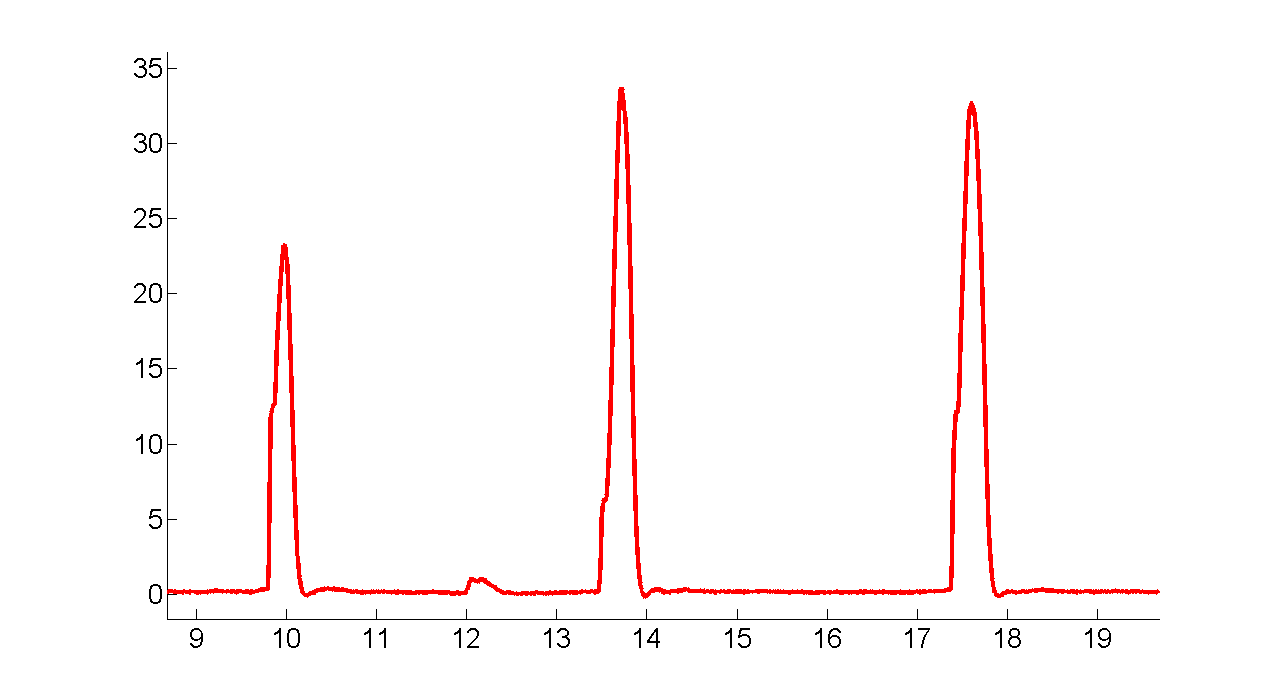
Identification Results changed with the data set. The green ones are from slow pushes data, red from fast pushes data and blue for normal pushes data.
As shown in the above figure and table,
- the mass and the position of the center of mass change with data set.
- the faster the push is, the higher the CoM tends to be.
In my experiments, I used M, CoM, Fext estimation for slow pushes, while MOI for fast pushes.
6 Download
Matlab code can be download here.
Footnotes:
1 Dynamic Parameter Identification for the CRS A460 Robot, Proceedings of the 2007 IEEE/RSJ International Conference on Intelligent Robots and Systems San Diego, CA, USA, Oct 29 - Nov 2, 2007
2 Robotics: Modelling, Planning and Control By Bruno Siciliano, Lorenzo Sciavicco, Luigi Villani, Giuseppe Oriolo
Date: 2009-11-11 13:52:42